The demand curve as perceived by a perfectly competitive firm is not the overall market demand curve for that product. However, the firm’s demand curve as perceived by a monopoly is the same as the market demand curve. The reason for the difference is that each perfectly competitive firm perceives the demand for its products in a market that includes many other firms; in effect, the demand curve perceived by a perfectly competitive firm is a tiny slice of the entire market demand curve. In contrast, a monopoly perceives demand for its product in a market where the monopoly is the only producer.
Total Cost and Total Revenue for a Monopolist
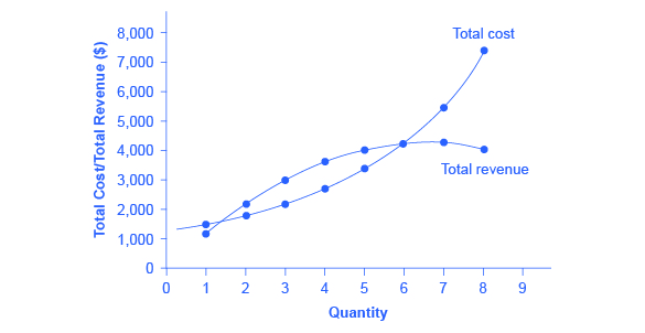
Profits for a monopolist can be illustrated with a graph of total revenues and total costs, as shown with the example of the hypothetical HealthPill firm in Figure 9.4. The total cost curve has its typical shape; that is, total costs rise and the curve grows steeper as output increases.

Figure 9.4. Total Revenue and Total Cost for the HealthPill Monopoly Total revenue for the monopoly firm called HealthPill first rises, then falls. Low levels of output bring in relatively little total revenue, because the quantity is low. High levels of output bring in relatively less revenue, because the high quantity pushes down the market price. The total cost curve is upward-sloping. Profits will be highest at the quantity of output where total revenue is most above total cost. Of the choices in Table 9.2, the highest profits happen at an output of 4. The profit-maximizing level of output is not the same as the revenue-maximizing level of output, which should make sense, because profits take costs into account and revenues do not.
| Quantity | Total Cost | Quantity | Price | Total Revenue | Profit = Total Revenue – Total Cost |
|---|---|---|---|---|---|
| 1 | 1,500 | 1 | 1,200 | 1,200 | –300 |
| 2 | 1,800 | 2 | 1,100 | 2,200 | 400 |
| 3 | 2,200 | 3 | 1,000 | 3,000 | 800 |
| 4 | 2,800 | 4 | 900 | 3,600 | 900 |
| 5 | 3,500 | 5 | 800 | 4,000 | 700 |
| 6 | 4,200 | 6 | 700 | 4,200 | 0 |
| 7 | 5,600 | 7 | 600 | 4,200 | –1,400 |
| 8 | 7,400 | 8 | 500 | 4,000 | –3,400 |
To calculate total revenue for a monopolist, start with the demand curve perceived by the monopolist. Table 9.2 shows quantities along the demand curve and the price at each quantity demanded, and then calculates total revenue by multiplying price times quantity at each level of output. (In this example, the output is given as 1, 2, 3, 4, and so on, for the sake of simplicity. If you prefer a dash of greater realism, you can imagine that these output levels and the corresponding prices are measured per 1,000 or 10,000 pills.) As the figure illustrates, total revenue for a monopolist rises, flattens out, and then falls. In this example, total revenue is highest at a quantity of 6 or 7.
Clearly, the total revenue for a monopolist is not a straight upward-sloping line, in the way that total revenue was for a perfectly competitive firm. The different total revenue pattern for a monopolist occurs because the quantity that a monopolist chooses to produce affects the market price, which was not true for a perfectly competitive firm. If the monopolist charges a very high price, then quantity demanded drops, and so total revenue is very low. If the monopolist charges a very low price, then, even if quantity demanded is very high, total revenue will not add up to much. At some intermediate level, total revenue will be highest.
However, the monopolist is not seeking to maximize revenue, but instead to earn the highest possible profit. Profits are calculated in the final row of the table. In the HealthPill example in Figure 9.4, the highest profit will occur at the quantity where total revenue is the farthest above total cost. Of the choices given in the table, the highest profits occur at an output of 4, where profit is 900.
Marginal Revenue and Marginal Cost for a Monopolist
In the real world, a monopolist often does not have enough information to analyze its entire total revenues or total costs curves; after all, the firm does not know exactly what would happen if it were to alter production dramatically. But a monopolist often has fairly reliable information about how changing output by small or moderate amounts will affect its marginal revenues and marginal costs, because it has had experience with such changes over time and because modest changes are easier to extrapolate from current experience. A monopolist can use information on marginal revenue and marginal cost to seek out the profit-maximizing combination of quantity and price.
The first four columns of Table 9.3 use the numbers on total cost from the HealthPill example in the previous exhibit and calculate marginal cost and average cost. This monopoly faces a typical U-shaped average cost curve and upward-sloping marginal cost curve, as shown in Figure 9.5. The second four columns of Table 9.3 use the total revenue information from the previous exhibit and calculate marginal revenue.
Notice that marginal revenue is zero at a quantity of 7, and turns negative at quantities higher than 7. It may seem counterintuitive that marginal revenue could ever be zero or negative: after all, does an increase in quantity sold not always mean more revenue? For a perfect competitor, each additional unit sold brought a positive marginal revenue, because marginal revenue was equal to the given market price. But a monopolist can sell a larger quantity and see a decline in total revenue. When a monopolist increases sales by one unit, it gains some marginal revenue from selling that extra unit, but also loses some marginal revenue because every other unit must now be sold at a lower price. As the quantity sold becomes higher, the drop in price affects a greater quantity of sales, eventually causing a situation where more sales cause marginal revenue to be negative.

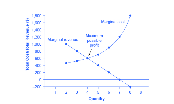
Figure 9.5. Marginal Revenue and Marginal Cost for the HealthPill Monopoly. For a monopoly like HealthPill, marginal revenue decreases as additional units are sold. The marginal cost curve is upward-sloping. The profit-maximizing choice for the monopoly will be to produce at the quantity where marginal revenue is equal to marginal cost: that is, MR = MC. If the monopoly produces a lower quantity, then MR > MC at those levels of output, and the firm can make higher profits by expanding output. If the firm produces at a greater quantity, then MC > MR, and the firm can make higher profits by reducing its quantity of output.
| Cost Information | Revenue Information | ||||||
|---|---|---|---|---|---|---|---|
| Quantity | Total Cost | Marginal Cost | Average Cost | Quantity | Price | Total Revenue | Total Revenue |
| 1 | 1,500 | 1,500 | 1,500 | 1 | 1,200 | 1,200 | 1,200 |
| 2 | 1,800 | 300 | 900 | 2 | 1,100 | 2,200 | 1,000 |
| 3 | 2,200 | 400 | 733 | 3 | 1,000 | 3,000 | 800 |
| 4 | 2,800 | 600 | 700 | 4 | 900 | 3,600 | 600 |
| 5 | 3,500 | 700 | 700 | 5 | 800 | 4,000 | 400 |
| 6 | 4,400 | 900 | 733 | 6 | 700 | 4,200 | 200 |
| 7 | 5,600 | 1,200 | 800 | 7 | 600 | 4,200 | 0 |
| 8 | 7,400 | 1,800 | 925 | 8 | 500 | 4,000 | –200 |
A monopolist can determine its profit-maximizing price and quantity by analyzing the marginal revenue and marginal costs of producing an extra unit. If the marginal revenue exceeds the marginal cost, then the firm should produce the extra unit.
For example, at an output of 3 in Figure 9.5, marginal revenue is 800 and marginal cost is 400, so producing this unit will clearly add to overall profits. At an output of 4, marginal revenue is 600 and marginal cost is 600, so producing this unit still means overall profits are unchanged. However, expanding output from 4 to 5 would involve a marginal revenue of 400 and a marginal cost of 700, so that fifth unit would actually reduce profits. Thus, the monopoly can tell from the marginal revenue and marginal cost that of the choices given in the table, the profit-maximizing level of output is 4.
Indeed, the monopoly could seek out the profit-maximizing level of output by increasing quantity by a small amount, calculating marginal revenue and marginal cost, and then either increasing output as long as marginal revenue exceeds marginal cost or reducing output if marginal cost exceeds marginal revenue. This process works without any need to calculate total revenue and total cost. Thus, a profit-maximizing monopoly should follow the rule of producing up to the quantity where marginal revenue is equal to marginal cost—that is, MR = MC.
If you find it counterintuitive that producing where marginal revenue equals marginal cost will maximize profits, working through the numbers will help.
Step 1. Remember that marginal cost is defined as the change in total cost from producing a small amount of additional output.
Step 2. Note that in Table 9.3 , as output increases from 1 to 2 units, total cost increases from $1500 to $1800. As a result, the marginal cost of the second unit will be:

Step 3. Remember that, similarly, marginal revenue is the change in total revenue from selling a small amount of additional output.
Step 4. Note that in Table 9.3 , as output increases from 1 to 2 units, total revenue increases from $1200 to $2200. As a result, the marginal revenue of the second unit will be:

Table 9.4 repeats the marginal cost and marginal revenue data from Table 9.3, and adds two more columns: Marginal profit is the profitability of each additional unit sold. It is defined as marginal revenue minus marginal cost. Finally, total profit is the sum of marginal profits. As long as marginal profit is positive, producing more output will increase total profits. When marginal profit turns negative, producing more output will decrease total profits. Total profit is maximized where marginal revenue equals marginal cost. In this example, maximum profit occurs at 4 units of output.
A perfectly competitive firm will also find its profit-maximizing level of output where MR = MC. The key difference with a perfectly competitive firm is that in the case of perfect competition, marginal revenue is equal to price (MR = P), while for a monopolist, marginal revenue is not equal to the price, because changes in quantity of output affect the price.
| Quantity | Marginal Revenue | Marginal Cost | Marginal Profit | Total Profit |
|---|---|---|---|---|
| 1 | 1,200 | 1,500 | –300 | –300 |
| 2 | 1,000 | 300 | 700 | 400 |
| 3 | 800 | 400 | 400 | 800 |
| 4 | 600 | 600 | 0 | 800 |
| 5 | 400 | 700 | –300 | 500 |
| 6 | 200 | 900 | –700 | –200 |
| 7 | 0 | 1,200 | –1,200 | –1,400 |