The purpose of selling costs is to influence the demand curve for the product of a firm or group. A producer incurs selling costs in order to push up his sales. Therefore, all selling costs tend to shift an individual seller’s demand curve to the right.
The question of a demand curve shifting to the left is altogether ruled out in this analysis. When the demand curve for the product of a firm shifts to the right, it is the result either of inducing the same customers to buy more of the same product or new customers buying this product attracted by the advertisement.
The new demand curve may be more or less elastic throughout its length or parts of it may be more or less elastic than the old demand curve before incurring selling costs. If the buyers are convinced of the superiority of this product in contrast with other similar products, the new demand curve will be less elastic in the upper segments than the old demand curve.
The firm will be losing few customers as a result of rise in the price of its product.
If, on the other hand, the old and the new customers are attracted more to the product, but, at the same time, are not prepared to pay a very high price, the new demand curve will be highly elastic in its lower portion.
Besides, the buying habits of the old and new customers also influence the shape of the demand curve. If they are influenced more by price changes rather than the product variation, the new demand curve will be highly elastic.
On the contrary, if they are not influenced much by price changes, the new demand curve will be less elastic than the old curve. In the analysis that follows straight-line demand curves are taken for the sake of simplicity.
When the new demand curve is drawn parallel to the old, the elasticity of demand on the higher curves is lower at each price. It means that the consumers are convinced of the superiority of this product and are willing to pay a higher price.
Price-Output Determination under Selling Costs:
Under monopolistic competition, an individual firm has a variety of choices to sell a larger output. It may do so by lowering the price of the product; it may improve its quality; it may indulge in greater sales promotion efforts or it may resort to all the three methods simultaneously or combine the one with the other. We shall, however be concerned with only selling costs.
But even this problem is complicated because to depict each level of output at each price and the possible AR, MR, MC, and AC curves on a two-dimensional figure become complex. So for the sake of simplicity, the demand curve and the average total cost curve are taken along with the average production cost curve.
The following analysis discusses the influence of the selling costs on the price-output policy of the firm and the group.
Firm’s Equilibrium under Selling Costs:
This analysis assumes that when a firm incurs selling costs:
(1) Its demand curve shifts upward to the right;
(2) The average total cost curve lies above the average production cost curve; and
(3) The firm maximises its net profits.
Since MC and MR curves are not shown in the diagram, the formula for calculating net profits is: Net Profits = (Price x Output)-(Production Costs + Selling Costs), i.e., the difference between the new demand curve and the average total cost curve multiplied by the number of units of the product sold at that price.
(1) Price Changes, Product and Selling Costs Remain Constant:
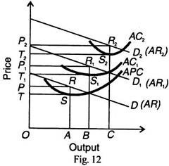
First we take the case of proportional selling costs with the assumption that only price change, sales remaining constant. The original demand curve is D (AR) and D1 (AR1) is the new demand curve. APC is the average production cost curve and AC is the average total cost curve, inclusive of selling costs.
The average total cost curve = average production costs + average selling costs. The firm maximises its output OQ at QA price and earns net profits measured by the area PRAT, as shown in Figure 11.
(2) Selling Costs Fixed, Price and Product Vary:
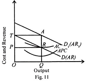
Suppose a firm spends Rs.1000 on advertising its product. Every time it spends this sum of money, the demand curve for its product shifts. In Figure 12, APC is the production cost curve and each time when Rs.1000 are spent on advertising, the average total cost curve becomes AC1 and AC2. D (AR) is the original demand curve before selling costs are incurred and D1 (AR1) and D2 (AR2) are the new demand curves.
The original equilibrium position is when OA output is sold at OP price. The firm earns TSRP super-normal profits.
Now, when selling costs are incurred in the first instance, the new equilibrium position brings T1S1R1P1 profits by selling OB output at OP1 price. Further expenditure of Rs.1000 on advertising increases profits to T2 S2 R2 P2, when ОС quantities of the product are sold at OP2 price.
The firm will, however, continue to spend Rs. 1000 on advertising its product each time so long as it adds more to total revenue than to total costs, till profits are maximised.
If the firm spends more on advertisement beyond this level, the addition to revenue will be less than costs. The firm will lose rather than gain by increasing selling costs. In Figure 12 the firm reaches the position of maximum profits when ОС product is sold at OP2 price and the firm earns T2S2R2P2 super-normal profits. Any further expenditure on advertisement will lead to diminution of profits.