The curve of selling costs is a tool of economic analysis forged by Prof. Chamberlain. It is a curve of average selling cost per unit of product. It is akin to the average cost curve and like the latter is U-shaped. Under the influence of the law of variable proportions, the curve of selling costs first falls, reaches a minimum point and then starts rising as shown in Figure 8.
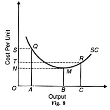
SC is the curve of selling costs. AQ is the average cost of selling OA units of the product, the total cost of selling it being OAQS. At the minimum point M of the SC curve, the cost per unit of selling OB units is BM which is less than any point in the QM portion of the SC curve. After this point, the average selling cost of ОС units is RC, the total cost of selling this quantity of the product being OCRT.
In fact per-unit selling cost and total selling costs increase beyond the minimum point M. According to Chamberlin, the shape of the curve and the exact point where it moves upward depends upon the nature of the product, its price, the nature of competing substitutes, the incomes of the buyers and their reluctance to change their tastes by the advertisement.
There is, however, a limit to the rising portion of the selling cost curve.
When the sales reach the saturation point, it ultimately becomes vertical. In the beginning, the application of successive doses of selling costs will raise the total sales more than proportionately so that average selling costs fall. This is due to two factors; firstly, consumers being attached to a particular brand of the product say, Brooke Bond Tea, are in the habit of buying it alone.
Advertisement in favour of another variety of the same product says Tata Tea, is meant to break their habit and dissolve the attachment of consumers to Brooke Bond Tea. One or two insertions a month in newspapers may make little impact on the consumers.
To convert the buyers to its brand, the manufacturer will have to incur larger selling outlays in the form of repetitive insertions of advertisement in newspapers, in commercial broadcasts, on the TV, in the form of samples, gifts or premium coupons.
Then only, sales will increase. Secondly, as larger outlays are incurred on sales promotion, internal economies of advertisement appear in the form of efficient salesmen, attractive advertisements and packing, etc. For instance, the larger the insertions and the size of advertisement, the lower the advertising rates per page. Thus, these two factors tend to lower average selling costs per unit of product up to a point.
Beyond this critical output M in our figure, average selling costs start rising again due to two forces. One, progressively increasing sales promotional expenses is to be incurred to induce regular consumers to continue to buy it.
Efforts to induce old customers to buy the same product require larger promotional expenses so that they are not only dissuaded from buying some other brand but also persuaded to buy more of the same product.
Two, larger selling outlays are required to attract new customers and those attached to other brands of the same product. They have to be convinced by repetitive advertisements in newspapers, through the radio, the cinema and television, of the superiority of this particular brand. Naturally such efforts require increased selling expenses.
As a consequence of these forces, average selling costs per unit of the product rise. We may conclude that two sets of forces operate in response to selling outlays on a product which tend to bring increasing returns up to a point, and beyond that, diminishing returns.
Proportional Selling Costs:
Average selling costs have the effect of raising the average total cost of production. If the average selling costs are proportional to the product sold, the curve of average total costs will lie at an equal distance above the average product cost curve.
For instance, when with a Signal toothpaste, a packet of five Erasmic blades is given free; the cost of five Erasmic blades incurred by the makers of the toothpaste represents proportional selling costs.
The product cost per unit of toothpaste and the selling cost per unit of a packet of blades added up from the total cost per unit of a tooth- paste-cum-five blade. The average production costs will rise by the cost of blades and will remain the same so long as the firm continues to sell in this proportion. This is illustrated in Figure 9 where APC represents the average production costs curve and AC the average costs curve.

The average costs are proportional throughout. They remain the same at all levels of output. At OQ output they are BA and even at OM level of output, they are the same as before DC (=BA), so is the average total cost MC (=QA). It should be noted that the corresponding MC curves of A PC and AC will also move in the same proportion (not shown in the figure).
We have assumed here that the producer continues to incur proportional selling costs which are unrealistic. In fact, a producer will resort to proportional selling costs only for a short while till his old stock is exhausted and in the process he also attracts new customers and induces regular users to buy more of it.
Fixed Selling Costs:
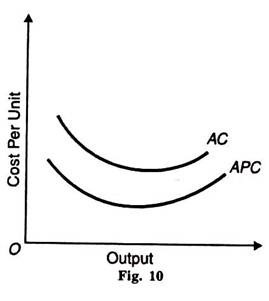
Selling costs are also of a fixed type, as in the case of screening a short-film in a cinema for a month or an insertion in the newspaper each Sunday. The average total cost per unit will at first be higher and as output increases it will fall and then, after a point, will start rising and the average total cost curve gradually becomes closer to the average production cost curve, as output increases further.
It implies that as sales increase, fixed selling costs are spread over a larger output and become less and less as shown in Figure 10, where APC represents the average production cost curve and AC the average total cost curve inclusive of selling costs.
The corresponding MC curves to APC and AC would be derived in the same manner and bear the same relation to their respective average cost curves. Added together they would give a combined MC curve (not shown in the figure).
Sometimes, certain tailoring and dry-cleaning concerns provide free home delivery service to their customers. But in such cases the effect of home delivery service is difficult to calculate on average and marginal costs.